Python charts with Matplotlib: lines, points and histograms

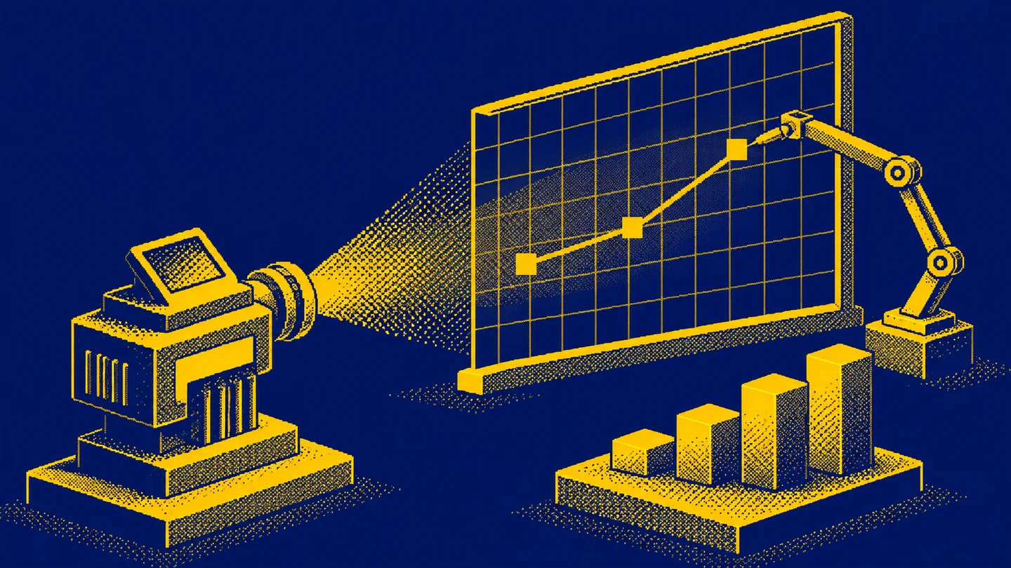
A Python chart takes only a few commands to produce. The harder question is what that chart lets you say about the data. I start there because it is easy to draw something impressive and only later discover a missing unit, points in the wrong order, or a line joining unrelated observations.

This guide introduces Matplotlib through small synthetic datasets. We will cover a line chart, a scatter plot and a histogram, then labels, scales and export. The syntax follows the Matplotlib 3.11 documentation. Each complete example includes its own imports and data. The editorial illustrations communicate ideas; they are not images produced by running the code.

Figure and Axes: a clear starting point

Matplotlib offers a function-based pyplot interface and a style that explicitly works with objects. The official quick start introduces both. I use fig, ax = plt.subplots() here because it remains easy to extend when another panel or data series is needed.

A Figure is the whole figure that you can save to a file. An Axes is the plotting area containing the data and its axes. The name can be confusing: an Axes is more than the individual horizontal axis. With one plot, subplots() returns one figure and one plotting area.

import matplotlib.pyplot as plt

period = [1, 2, 3, 4]
orders = [10, 14, 12, 18]

fig, ax = plt.subplots(figsize=(8, 4), layout="constrained")
ax.plot(period, orders, marker="o")
ax.set(
    title="Orders across four periods: synthetic data",
    xlabel="Period",
    ylabel="Number of orders",
)
ax.set_xticks(period)
plt.show()

This assumes Matplotlib is available in the environment running the code. If the import fails, I check that environment first. A notebook and a terminal can use different Python interpreters. Installing a package in whichever terminal happens to be open does not guarantee that the notebook can import it.

figsize sets the figure size in inches. layout="constrained" helps fit labels within the figure. You still need to inspect the output: a long title or a large legend can change how readable the whole composition is.

When connecting points makes sense

The periods in the example are ordered, and each count represents orders in the next comparable period. A line helps track the movement from 10 to 14, down to 12, and up to 18. Markers show where the observations actually sit.

Having only a few points does not automatically make a line chart inappropriate. Four monthly observations can form a useful short series. The more useful question is what the connection means: is the order natural, and will readers understand that the segment between measurements is not another measurement?

The Axes.plot documentation describes drawing lines and markers. Points are connected in the order supplied. If an export lists dates out of order, arrange the observations before plotting. The chart cannot establish the intended business sequence for you.

I would avoid joining successive customers merely because their identifiers run from 1 to 100. That segment implies continuity that the numbering does not establish. For a few categories I would consider bars; for the relationship between two quantitative variables I would consider a scatter plot.

Scatter plots: one pair of values per observation

Take four synthetic parcels. I want to examine the relationship between parcel weight and packing time. Each point represents one parcel, without connecting it to the next parcel.

import matplotlib.pyplot as plt

weight_kg = [1, 2, 3, 4]
packing_minutes = [3, 4, 4, 7]

fig, ax = plt.subplots(figsize=(8, 4), layout="constrained")
ax.scatter(weight_kg, packing_minutes, s=60)
ax.set(
    title="Weight and packing time: synthetic data",
    xlabel="Parcel weight [kg]",
    ylabel="Packing time [min]",
)
plt.show()

Two parcels have a packing time of four minutes, and the heaviest parcel has the longest time. These four invented observations demonstrate how to read the plot; they do not establish a conclusion about a warehouse. The arrangement also does not prove that greater weight causes slower packing. Box size, product type and the packer’s experience could matter.

In Axes.scatter, s specifies marker area in points squared. Doubling s does not double the diameter. Initially, I keep marker size constant rather than introduce another way of encoding information without a clear reason.

With many observations, points can overlap. Smaller markers and transparency can help, but a styling change alone does not tell you how many records sit underneath a single visible point. Check the distribution and counts in the underlying data as well.

Histograms describe one variable’s distribution

A histogram answers a different question: how often do values fall into successive intervals? Instead of two coordinate lists, I need one list of measurements. Here are handling times for six synthetic support requests:

import matplotlib.pyplot as plt

minutes = [1, 2, 2, 4, 5, 7]
edges = [0, 3, 6, 9]

fig, ax = plt.subplots(figsize=(8, 4), layout="constrained")
ax.hist(minutes, bins=edges, edgecolor="black")
ax.set(
    title="Request handling time: synthetic data",
    xlabel="Handling time [min]",
    ylabel="Number of requests",
)
ax.set_xticks(edges)
plt.show()

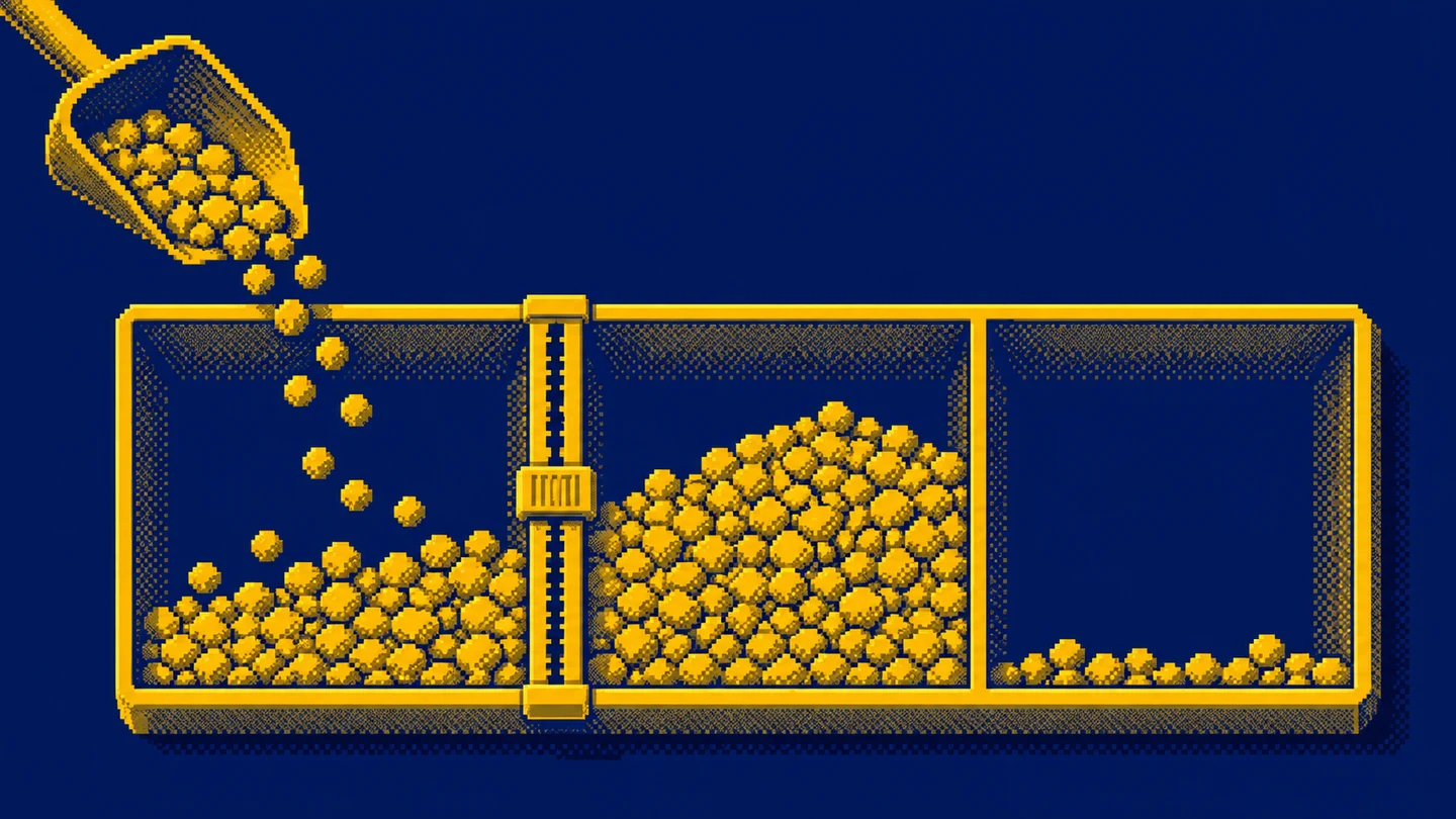
We can trace the counts manually. The first interval includes 0 and excludes 3. It contains 1, 2 and 2, so its height is 3. The second interval starts at 3 and excludes 6. It contains 4 and 5, giving a height of 2. The final interval includes both 6 and 9. It contains 7, giving a height of 1. That accounts for all six requests.

These boundaries follow the hist documentation: all bins except the last are closed on the left and open on the right. The last includes both endpoints. An observation of exactly 3 would therefore enter the second bin, while an observation of 9 would enter the final one.

The choice of bins changes the picture

The default number of histogram bins is 10. That default is a starting setting rather than an analytical justification. Ten bins for six observations can break the picture into mostly empty fragments. Too few bins for a much larger sample can hide useful differences.

I first choose boundaries that make sense for the measurement, then check whether a modest change alters the overall conclusion. If the entire story disappears when one boundary moves, it needs more cautious wording. When comparing two groups, I keep the same boundaries so the apparent difference does not come only from settings.

All measurements in our example lie inside the supplied boundaries. Custom boundaries can leave observations outside the histogram. Before interpreting the bar heights as a complete population, I check the range and the number of included observations. This is particularly easy to overlook after applying a filter.

Setting density=True changes the vertical axis to density. The histogram’s area is normalised; simply adding the heights does not necessarily give one. For a first report with a small sample, I keep counts because they are easier to explain. With unequal bin widths, I explicitly state whether the chart represents counts or densities.

Titles, labels and units do analytical work

A title such as “Analysis” tells me very little. I prefer “Request handling time”, and in a real report I add the period and scope: which requests and which source system. Units distinguish seconds from minutes, gross from net values, and orders from individual products.

I label synthetic inputs explicitly. For an actual business report, I describe the source and refresh time beside the chart or in its caption. Readers should be able to tell whether they are seeing a complete month, part of a month, or a comparison limited to equivalent working days.

ax.set_xticks(period) places ticks at the selected period values. It does not change observation coordinates or filter records. This avoids distracting fractional period labels, while leaving you responsible for what the numbers in period mean.

A second series needs useful names and a legend. Colour helps distinguish series, but should not carry the entire explanation. Different markers or direct labels near a line can be easier to use, especially when the chart is printed in greyscale.

Linear and logarithmic scales

I choose a logarithmic scale when the question concerns proportional changes across a wide range of positive values. Equal distances then represent equal ratios, such as successive tenfold increases. On a linear axis, equal distances represent equal differences.

For an existing plotting area ax, the change is:

ax.set_yscale("log")

This line modifies an existing chart; it is not a complete standalone program. Add it before saving or displaying the figure. The order counts in our first example range only from 10 to 18, so a linear scale is sufficient. A log scale would add complexity to a straightforward comparison.

The standard LogScale is for positive values. Zeros and negative values need deliberate treatment; the library can mask or clip them depending on the configuration. I avoid adding one to every value without explanation because that changes the data’s meaning. If negative values matter, I reconsider the scale and presentation.

Display a chart and save a file

plt.show() requests display of open figures. Behaviour depends on the environment and backend. A notebook may display the result beneath a cell, a script may open a separate window, and a server without a graphical interface may be better served by saving a file.

For the fig created in the first example, add this before show():

fig.savefig("orders.png", dpi=150, bbox_inches="tight")

Figure.savefig saves that particular figure. The extension selects PNG here. The path is relative to the working directory, and an existing file with the same name may be replaced. Use a separate practice directory and deliberately choose the output name.

An 8 by 4 inch figure at 150 DPI has a basic canvas of 1200 by 600 pixels. bbox_inches="tight" adjusts the exported region to the content, so final dimensions may differ. If a recipient requires exact dimensions, establish those requirements separately and inspect the resulting file.

The show documentation also explains saving order: a blocking display can close and unregister the figure from pyplot. Retaining the fig reference gives more control. In a simple script, I consistently prepare the plot, label it, save it, and then display it.

What I check before sharing a chart

First I return to the input. Is every observation counted once? Do both lists refer to the same records in the same order? If parcel weights come from one sort and handling times from another, the scatter plot can look plausible while displaying invented pairs.

Then I check coverage: missing values, filters, incomplete periods and measurements outside configured boundaries. An empty plot can signal a filter or data-type problem. Titles and colours cannot repair source preparation errors. The introductory pandas reporting project is a useful next step for that preparation.

Finally, I view the exported file at the size the recipient will actually use. A chart readable on a wide monitor can have tiny labels once placed in a document. I shorten the title, remove decoration and confirm that the unit remains visible. If interpreting the result needs several sentences, I write them alongside the chart instead of forcing the entire analysis into the legend.

I also look for a mismatch between the title and the population. A chart titled “Customer demand” might actually count support tickets, repeated requests or attempted orders. Before discussing a trend, I describe the counted unit precisely. That small wording choice can prevent an otherwise polished graphic from answering a different question than the reader expects.

For repeated reporting, I keep a consistent definition of periods and groups. Moving from calendar weeks to rolling seven-day windows changes the comparison, even if the line colour stays the same. A visually consistent dashboard still needs consistent measurement rules behind it. When a definition changes, I make the change visible in the report rather than let readers infer continuity.

A missing measurement and a zero tell different stories

Suppose the source system did not deliver data for the second period. Entering zero in its place suggests that no orders occurred. That is a much stronger claim than saying the result is unknown. I first establish whether the measurement is unavailable or merely awaiting an update. The gap should remain understandable to someone who sees only the exported chart.

Monthly comparisons have a similar trap. If one month includes all days and another includes only its first few days, joining their totals can create an apparent decline. I label the incomplete period or compare the same range of days. I also keep any forecast visibly distinct from observed values.

Changes in units deserve the same attention. If an earlier export measured time in seconds and a new one uses minutes, the chart can suggest a sudden improvement. The library does not know what the number 60 means. A column definition establishes whether it represents minutes, hours, items or a percentage. I establish the unit while preparing data and use the label as visible confirmation.

When two series appear in separate panels, I inspect their axis ranges. Independent automatic scaling can make a small and a large movement occupy similar heights. Depending on the question, a shared scale may help, but both series need inspection. I first decide whether the comparison concerns absolute levels or the shape of change.

Histograms and category bars answer different questions

The three histogram columns in our example represent time intervals, with an order determined by a numeric axis. Columns labelled “phone”, “email” and “chat” would represent contact-channel categories. I prepare category counts for that comparison and use a bar chart. Feeding category numbers into a histogram would leave their meaning unexplained.

Imagine five contacts: two by phone, two by email and one by chat. A channel comparison concerns those three counts. A handling-time analysis could place the same contacts into entirely different time groups. Changing the chart type here also changes the question being answered.

Before aggregation, I check the counted unit. One contact may cover several topics, while a single support request may contain several contacts. If the goal is to count requests, a message-level export needs an appropriate request identifier. A well-chosen histogram cannot fix a mismatch in the level of detail.

For recurring reports, I keep the observation and bin definitions with the plotting code. Someone updating the report next month should understand why a boundary is three minutes and what the final interval includes. These small decisions make the code a readable account of the analysis and help the chart retain its meaning when another person takes over.

Exercise: three questions, three chart choices

Plot the synthetic order counts across four periods. Write one sentence explaining what the segment between observations represents. Next, prepare the parcel weight and packing time scatter plot. Note one possible explanation for the relationship and one question the chart cannot settle.

Finally, recreate the histogram of six handling times. Count the observations in the three intervals manually before running your own version, then move the boundary from 3 to 2. Pay attention to measurements equal to a boundary. This small exercise shows how much meaning can sit inside the single bins parameter.

Save each chart with units, a synthetic-data label and a one-sentence description. I would consider that a useful first result: you can choose a chart, explain its input and give someone a file they can read without guessing.