KajoData / statistics
The Gaussian curve: normal distribution and its limits
I explain model probabilities and why a bell curve alone cannot validate data or forecast future performance.
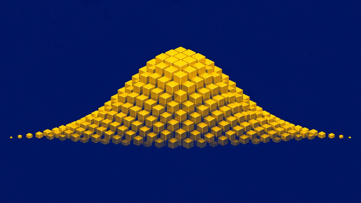
The Gaussian curve appears so often that it can start looking like the default shape of every dataset. I treat it as a specific model that needs to fit the question and be checked. Calculating a mean and standard deviation does not make handling times, grades or revenues normally distributed. It is possible to draw a beautiful bell over data that it describes badly.
I will explain what the model actually says, how to interpret the familiar 68-95-99.7 rule, and when to pause before applying a ready-made formula. The examples are synthetic. Their purpose is to explain the mechanism, rather than establish that a real process must be normal. That distinction is often more useful than knowing how to draw the curve itself.
What the normal distribution is
The normal distribution is a continuous probability distribution. Its probability density has a symmetric shape, one central peak and a tail on either side. The model’s mean, median and mode coincide. The mean sets the centre and a positive standard deviation sets the scale. NIST describes these properties in its distribution reference.
“Gaussian curve” usually refers to this density plot. However, not every symmetric mound is normal. Other symmetric distributions have different tails and assign different probabilities to distant values. A visual resemblance may be a useful starting point, but it does not complete the assessment. When a decision concerns rare events, the tails can matter more than the appearance of the central peak.
The word “normal” does not mean correct, desirable or universal. A completion time can be measured correctly and still be strongly skewed. A complaint count can be valid and discrete. I do not try to repair such data merely to make them resemble a textbook picture. First I ask which process generated the observations and which values are possible in that process.
Probability is area rather than point height
For a continuous distribution, probability corresponds to the area under the curve over an interval. The total area equals one. The curve’s height at a point is a density, rather than the percentage of observations with exactly that value. In the continuous model, a single exact value has probability zero. Intervals are meaningful even when everyday language asks about a particular result.
If a measurement is recorded to the nearest whole unit, a displayed value of 100 can represent a range of underlying values after rounding. That differs from the mathematical point exactly equal to 100. In a report, I pay attention to measurement precision and histogram bin widths. Two similarly worded questions can require different calculations when one concerns an interval and another concerns a rounded recorded value.
What the mean and standard deviation change
Suppose the model has a mean of 100 and a standard deviation of 10 in arbitrary measurement units. Its centre is at 100. Changing the mean to 120 shifts the bell to the right. Changing standard deviation from 10 to 20 widens the curve and lowers its peak, because its total area must remain one. A wider bell does not have more total probability.
Parameter notation requires care. Statistics often uses N(μ, σ²), with variance as the second parameter. A library may instead ask for standard deviation as a scale parameter. SciPy documents loc as the mean and scale as standard deviation. Our example has variance 100 but scale 10 in that interface. Passing 100 instead of 10 specifies a very different model.
The one, two and three standard deviation rule
Under a normal model, fixed distances from the mean contain fixed proportions of the distribution. NIST gives approximately 68.27%, 95.45% and 99.73%. These are often remembered as 68-95-99.7. They are properties of the model, rather than a guarantee that precisely those percentages of rows in any dataset will fall inside the intervals.
| Model interval | With mean 100 and standard deviation 10 | Proportion |
|---|---|---|
| mean ± 1 standard deviation | 90 to 110 | approximately 68.27% |
| mean ± 2 standard deviations | 80 to 120 | approximately 95.45% |
| mean ± 3 standard deviations | 70 to 130 | approximately 99.73% |
About 4.55% lies outside the second interval, split equally into approximately 2.275% in each tail. A value above 120 is therefore not an error by definition. The model itself allows such observations. Assessing a particular measurement also requires the variable’s meaning, source quality and response rules. A statistical threshold does not replace knowledge of what the process can produce.
Standardization connects values to the model
Calculate a z-score as z = (x - μ) / σ. With x = 120, μ = 100 and σ = 10, the result is z = 2. With x = 90, it is z = -1. This states how many standard deviations separate a point from the centre and on which side it lies. It allows use of the standard normal distribution, whose mean is zero and standard deviation is one.
Calculating a z-score does not require every input column to be normal. Assigning normal-model probabilities to that score does require an appropriate model. This is a common confusion: subtracting the mean and dividing by standard deviation does not magically turn the distribution into a bell. If the original data have two peaks, an ordinary linear standardization will not combine them into one.
The cumulative distribution answers threshold questions
The cumulative distribution function F(x) gives the probability of a value less than or equal to x. At the normal model’s mean it equals 0.5, because half the area lies to the left. The probability of exceeding x is 1 - F(x). For the interval from a to b, subtract F(a) from F(b). This separates a question about the upper tail from one about both tails together.
Our interval from 80 to 120 contains about 95.45%, but the area to the left of 120 is larger. It includes that central interval and the lower tail. By symmetry, it is approximately 97.725%. Confusing the two questions gives the wrong answer even with the correct mean and standard deviation. Before choosing a function, I write whether I need values below a threshold, above it or between two boundaries.
The SciPy norm documentation separates density pdf, cumulative probability cdf and the upper-tail survival function sf. Similar names answer different questions. I would not interchange them because the associated plots look familiar. Symmetry and the stated area proportions are enough to understand the distinction on paper. In an actual calculation I also check units, parameter scale and whether the threshold concerns an individual observation or a mean.
Known parameters and estimated parameters
So far, I have treated 100 and 10 as the model’s specified parameters. In real analysis, I usually estimate them from data. The resulting interval is then based on estimates and carries additional uncertainty. Three observations cannot support unrestricted claims about the tails of a large process. With limited information, I interpret precise-looking percentages cautiously.
I also separate the standard deviation of observations from the standard error of the mean. The first describes variation among individual measurements. The second concerns uncertainty in the mean estimator. NIST discusses confidence intervals for the mean separately. An interval containing about 95% of model values is not automatically a 95% confidence interval for the mean. They answer different questions and need different labels.
Begin the assessment with a histogram
A histogram helps reveal asymmetry, multiple clusters, gaps and long tails. I pay attention to bin width: wide bins can conceal two peaks, while very narrow bins can emphasize random irregularities in a small sample. NIST describes histograms as a tool for inspecting distribution shape. I do not treat one display setting as a final verdict.
I also establish the observation level. A histogram of daily means differs from a histogram of individual transactions. Both may be valid, but they describe different levels. If I care about the risk of an unusually long individual case, daily means may hide it. Before debating normality, I state the unit of analysis and the filter that selected the chart’s input.
A Q-Q plot reveals departures from the model
A normal Q-Q plot compares data quantiles with normal-distribution quantiles. When the model is a reasonable approximation, points lie roughly along a straight line. Systematic curvature or departures at the ends show where further investigation is needed. NIST explains the normal probability plot and the role of deviations from a line.
I do not expect a finite sample to form a perfect line. Random data have random irregularities. Instead, I ask whether a discrepancy is large enough, and in a relevant enough region, to affect the decision. If the calculation concerns an extreme tail, a modest departure at the end can matter more than an excellent fit in the centre. The analytical objective determines the accuracy required.
A normality test does not finish the analysis
A formal test, such as Shapiro-Wilk in the SciPy documentation, can complement plots. Failing to reject normality does not prove that the distribution is perfectly normal. A small sample may provide limited information about departures. A large one may reveal a slight discrepancy that has little practical effect on a particular application.
I do not choose a model from one p-value alone. I consider the plots, the collection process and the requirements of the subsequent method. Comparing means requires checking the assumptions of the selected procedure, including independence. Estimating rare exceedances requires particular attention to the tails. The same small departure can have different consequences for two different questions.
The central limit theorem concerns means
A common shortcut says that a large sample makes the data normal. That is misleading. In the classical central limit theorem, the object is the appropriately standardized mean of independent, identically distributed observations with finite positive variance. Penn State’s teaching material distinguishes the variable from its sample mean. Original observations can remain skewed even as a normal approximation for the mean becomes useful.
There is no universal magic sample size that removes every problem. Strong skewness, heavy tails and dependence require attention. Adding thousands of dependent rows does not automatically justify a formula intended for independent sampling. First I establish the sampling method and what each record represents. Only then do I ask whether a normal approximation is adequate for the calculation being planned.
Mixed groups can create two peaks
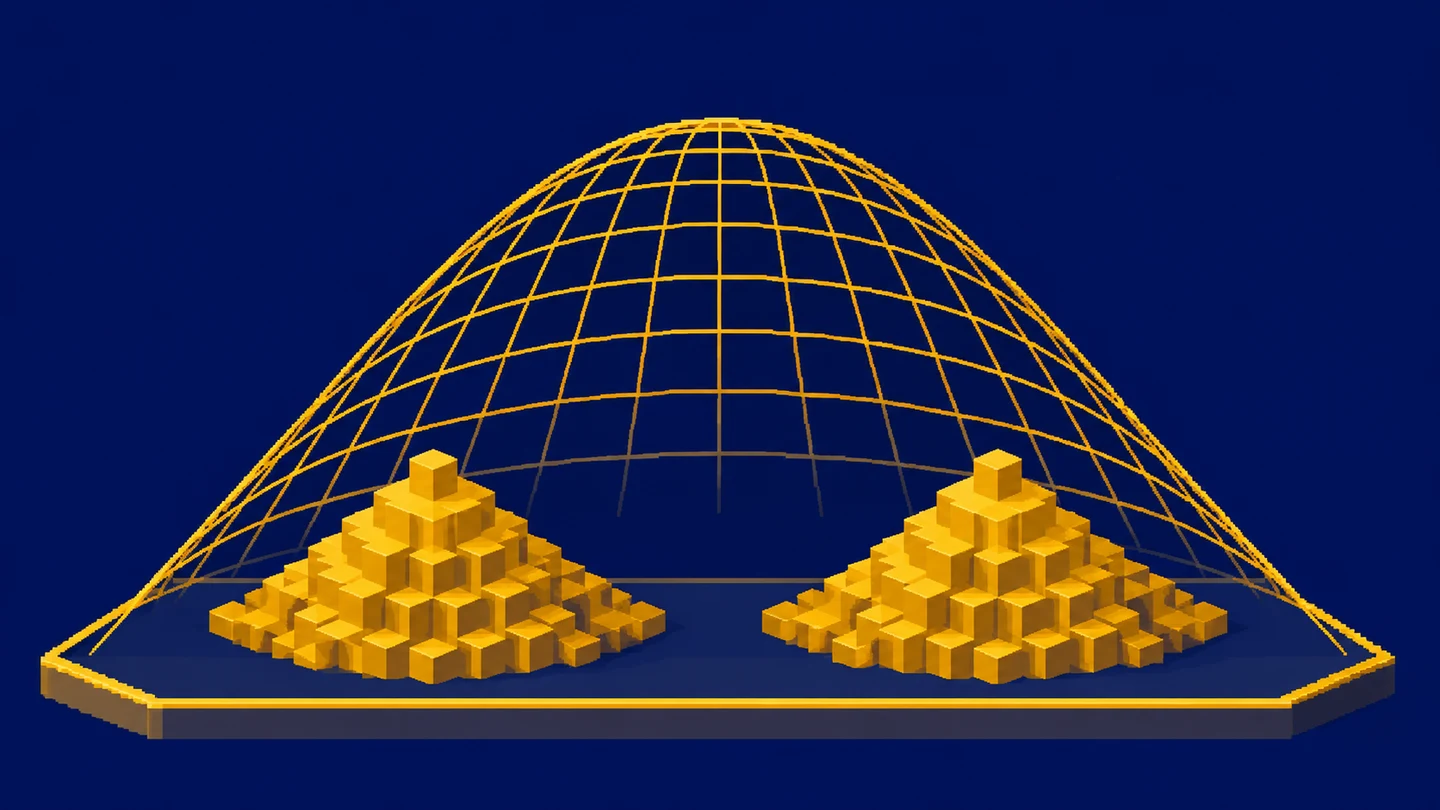
Imagine two measurement stations. One produces values concentrated near 90 and the other near 110. Their combined mean may be near 100, where there need not be many observations at all. Overlaying one bell with a shared mean would hide the two-group structure. This synthetic scenario shows why source labels deserve inspection before fitting one curve to everything.
Products, shifts or handling methods can create similar situations. Separating groups is analytically relevant when each represents a different process. I still check that the split has a substantive explanation, rather than merely improving the fit. Dividing the data repeatedly until an attractive bell appears can create a convenient story that no longer describes the original collection honestly.
Variable boundaries and changes over time
A normal distribution permits all real values. Duration cannot be negative, while a case count is nonnegative and discrete. The normal model may sometimes approximate a useful range, but I check how much probability it assigns to impossible outcomes. If the model frequently predicts negative durations, that is a serious sign that it does not suit the task.
I assess process stability separately. Last year’s mean and dispersion may no longer describe the situation after a system or policy change. A distribution has no time axis and cannot, by itself, predict future development or performance a decade later. Forecasting needs assumptions about changes and a method appropriate to time-dependent data. An attractive bell does not supply those ingredients.
Statistical significance needs a specific hypothesis
I do not test whether “the data are statistically significant.” A test concerns a specific hypothesis and statistic, with an interpretation that depends on assumptions. Normal distributions appear in many methods, but a bell on a chart does not establish practical importance. A large sample can detect a difference too small to change any useful decision.
Before testing, I would specify the comparison, analysis level and practically important difference. Then I would check whether the data and procedure can answer that question. Numerical interpretation comes after those choices. This avoids inventing a story around a p-value found after trying many alternatives. A distribution also cannot establish whether an observed association is causal.
Write a conclusion that matches the evidence
Rather than declaring all the data normal, I would identify the variable and range for which the model is an approximation and where it fits poorly. I would show the sample size, parameters, units and a plot. If I use the standard-deviation percentages, I state that they come from the model. The observed fraction of records in that interval is a separate quantity, rather than the same number by definition.
When the model fits poorly, I can still describe the data with a median, quartiles and IQR and appropriate quantiles. Standard deviation can also be calculated descriptively without claiming normality. Choosing a method for further inference is another decision. An overly simple first model does not make the entire analysis a failure.
An interpretation exercise
For a model with mean 100 and standard deviation 10, write the two-standard-deviation interval. It is 80 to 120. Now ask whether every observation must lie inside it, whether 125 must be a mistake, and whether a million observations necessarily make the original variable normal. Each answer is no, but for a different reason.
Explain those reasons in your own words: the model has tails, record validity needs context, and the central limit theorem concerns a mean’s distribution under assumptions. Then inspect one of your reports and check whether any fitted bell is supported by examining the data. That is where I would begin learning to use the normal distribution at work. Naming a limitation can be more useful than another decimal place.
Key takeaways
What determines a normal distribution?
The mean sets its location and a positive standard deviation sets its scale. The model has equal mean, median and mode.
Does standardization make data normal?
Subtracting the mean and dividing by standard deviation changes scale but does not remove skewness or multiple peaks.
Does a large sample mean normal observations?
The central limit theorem concerns the distribution of an appropriately standardized sample mean under assumptions, rather than changing the original observations into normal data.
AI was used in an automated way while working on this article. If you want to learn how to do it too, check out this project.